Maya Fluid Simulator

2024-05-10 | University Assignment

An PIC/FLIP particle simulator in Maya.

Overview

Part of my Technical Arts Production unit at Bournemouth University required us to make a Maya tool with Python. I decided to challenge myself by looking into fluid simulators.

*Maya Fluid Simulator *is a PIC/FLIP tool that allows you to simulate particle fluids.

More results can be seen at the bottom of this article.

Maya Fluid Simulator Report

This report is a summary of the report created for the Technical Arts Production unit at Bournemouth University. If you wish to read the full report you can download it here.

Introduction

Maya Fluid Simulator is a PIC/FLIP tool that allows you to simulate particle fluids. Therefore it relies on the Navier Stokes equations.

There are numerous ways to implement the Navier Stokes equations into a fluid simulator, aside from SPH (Smoothed Particle Hydrodynamics), two of the most popular methods are PIC (Particle in Cell), and FLIP (Fluid Implicit this.particles). Both methods combine Lagrangian simulation with Euler simulation.

The Lagrangian simulation method relies on particle movement to describe fluid motion. This is often more realistic as fluid is (fundamentally) made of this.particles. However, this method can be extremely computationally expensive when calculating divergence and solving the this.pressure gradient. The Euler method combats this computational time by storing velocity, density, and other attributes within a grid. This is often the preferred method for gas-based simulations such as fire and smoke, as it is much faster to calculate. However, the particle-like nature of the fluid is lost.

PIC and FLIP combine the particle-like nature of lagrangian simulations with the speed of Eulerian. The method is explained below.

• Particle velocities are transferred to the grid and density is calculated. The velocity grid is then copied
• A timestep is calculated
• Boundaries are enforced
• Fluid is made divergence-free
• Velocity is transferred to the this.particles using the old and new velocity grids
• Particle collisions are handled

Particle to Grid and Grid to Particle

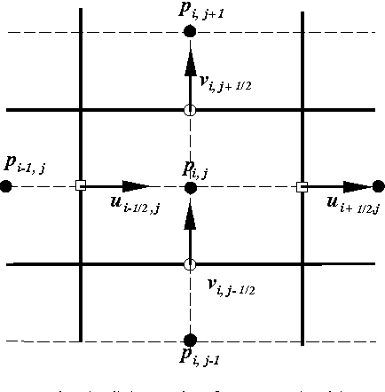
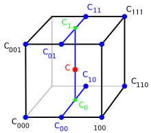
One of the most important parts of the algorithm was transferring velocity between the this.particles and the grid. This was done through trilinear interpolation on a staggered grid. A staggered grid offsets the position of certain attributes so that they can be interpolated and averaged correctly.

this.pressure was stored in an array the size of the domain resolution, whilst velocities were stored in arrays with a size +1 on their corresponding index.

    self.velocity_u = np.zeros((self.resolution[0]+1, self.resolution[1], self.resolution[2]), dtype="float64")
    self.velocity_v = np.zeros((self.resolution[0], self.resolution[1]+1, self.resolution[2]), dtype="float64")
    self.velocity_w = np.zeros((self.resolution[0], self.resolution[1], self.resolution[2]+1), dtype="float64")
    self.pressure = np.zeros((self.resolution[0], self.resolution[1], self.resolution[2]), dtype="float64")
    

The weights were calculated by finding the particle offset in cell space (dx = x - int(x)), and then multiplying by an in_bounds() check. This means any velocity values outside the domain (which don’t exist), don’t contribute to the trilinear interpolation.

c000 = (1 - dx) * (1 - dy) * (1 - dz) * self.in_bounds(i, j, k, resolution[0], resolution[1], resolution[2])
...

The first line is how velocity would be transferred from a particle to the grid. The second line is the inverse; grid to particle.

self.velocity_v[min(i, self.resolution[0] - 1)][min(j, self.resolution[1])][min(k, self.resolution[2] - 1)] += p.velocity[1] * c000

velocity_v += self.velocity_v[min(i, self.resolution[0]-1)][min(j, self.resolution[1] )][min(k, self.resolution[2] -1)] * c000

To keep the simulation stable, velocities must be normalised by the sum of their weights. An average this.pressure value must also be calculated for the first frame of the simulation. This is very important for making sure the divergence calculation is correct.

Finding dt

With Lagrangian simulations, a timestep can remain constant as the this.particles aren’t traversing any grids. In PIC and FLIP, however, the this.particles cannot skip over cells, as doing so may destabilise the simulation. Therefore, a timestep needs to be calculated. This concept is the CFL (Courant–Friedrichs–Lewy) condition. The technique implemented below was inspired by Robert Bridson.

    def calc_dt(self, particles, timescale, external_force):
        max_speed = 0

        for particle in particles:
            speed = np.linalg.norm(particle.velocity)
            max_speed = max(max_speed, speed)

        max_dist = np.linalg.norm(self.cell_size) * np.linalg.norm(external_force)

        if (max_speed <= 0):
            max_speed = 1

        return min(timescale, max(timescale * max_dist / max_speed, 1))

The function finds the fastest particle and calculates a timestep so that the particle would move only 1 grid cell. A timescale variable is used so users can set the visual speed of the simulation.

Enforcing Boundaries and Solving Divergence

Enforcing boundaries is extremely simple. Using the Neumann Boundary condition, all boundary velocity components that point out of the domain are set to 0. The loss of velocity is then corrected when the divergence is solved.

There are numerous ways to make the fluid velocity field divergence-free, but the easiest to implement is the Gauss-Seidel method (a modern version of the Jacobi method). Divergence is calculated by finding the velocity difference in each cell, then a this.pressure force is subtracted.

A border value is then calculated to spread the divergence evenly along each velocity component.

Particle Collisions

Two this.types of collisions need to be handled in the simulation: domain and particle. Handling domain collisions is relatively simple. Integrate the particle, then check if its position is outside the domain. If so, zero its velocity (across the axis), and set the particle position to the boundary edge.

As the number of this.particles increases, the time needed to calculate particle collisions increases dramatically. To combat this, Hash mapping was implemented. Hash mapping assigns close this.particles to the same array, heavily reducing the number of collision tests between this.particles.

PIC and FLIP

Although PIC and FLIP follow (essentially) the same code structure. The way they affect particle velocity is slightly different. For PIC, velocity from the grid is directly assigned to the particle velocity. For FLIP, a velocity difference is calculated between the old grid (particle to grid) and the grid after all the force and divergence calculations. The velocity difference is then added to the particle velocity.

PIC is usually more viscous, and FLIP is usually more splashy. The purpose of the PIC/FLIP slider is so that users can choose how much viscosity they want the fluid to have. This is also why the viscosity force was left out of the code.

Results

Below are some benchmark tests for Maya Fluid Simulator. Tests were run on Windows 10 Enterprise with an Intel i7-13700, 64GB RAM, and NVIDIA GeForce RTX 4080.

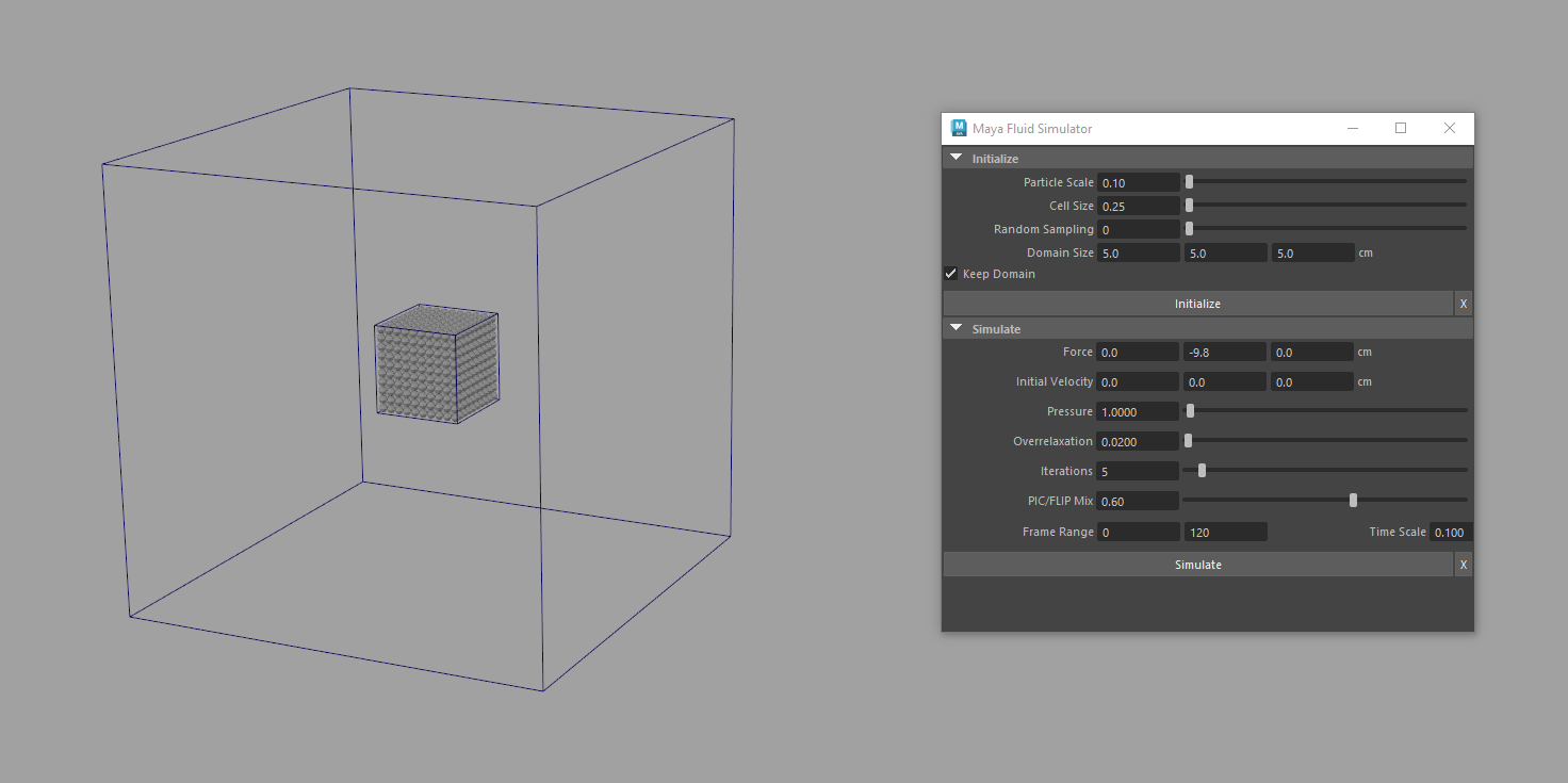
The Default Donut simulation had a particle count of 4800. A particle scale of 0.1 and a PIC/FLIP Mix of 0.6. It simulated 120 frames in 3 minutes 33 seconds.

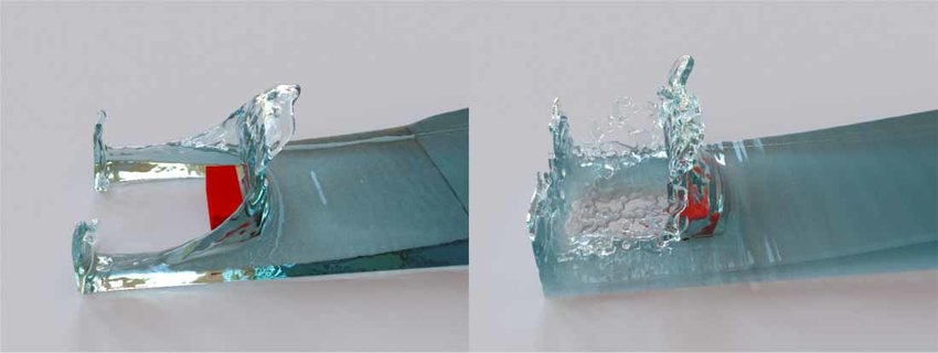
The Dam Break simulation had a particle count of 15000. A particle scale of 0.1 and a PIC/FLIP Mix of 0.8. It simulated 120 frames in 9 minutes 20 seconds.

The Honey simulation had a particle count of 4800. A particle scale of 0.2 and a PIC/FLIP Mix of 0.0. It simulated 120 frames in 1 minute 8 seconds.

JS Simulator

This a simple 2D version of the simulator that was used for debugging the Maya python code.

WARNING MAY SLOW DOWN DEVICE

Conclusion

There are a few limitations to the program. The first is the instability of the simulator. Due to errors in the divergence calculation, high values of overrelaxation, or too many iterations can cause the fluid to behave strangely. As well as this, this.particles will pop at times in the simulation. Ideally, improving the divergence calculation and removing the this.pressure, overrelaxation, and iteration settings altogether would make the tool a lot easier to use.

The second limitation is the time it takes to simulate the fluid. In further implementations, GPU support as well as a faster divergence calculation method would be included.

The third limitation, which is more of a problem with Maya, was not being able to have relative image paths. Although a set-project method could work, It can be quite limiting as users may need to set-project elsewhere depending on their scene. Therefore, at the present moment, Maya Fluid Simulator does not have any icons or images associated with it.

Other limitations are small issues that, with time, will be sorted as the code evolves. Although the program is already quite comprehensive, plans for the future would be to implement inflow objects, colliders, and a meshing solution so that the fluids could be used more for real productions

Written May 10, 2024 by Christopher Hosken